
Work with Computer Vision: Monitor Traffic in Norway
I haven’t ventured out of natural language processing much, but I have wanted to write about using computer vision for some time, specifically with a practical use case.
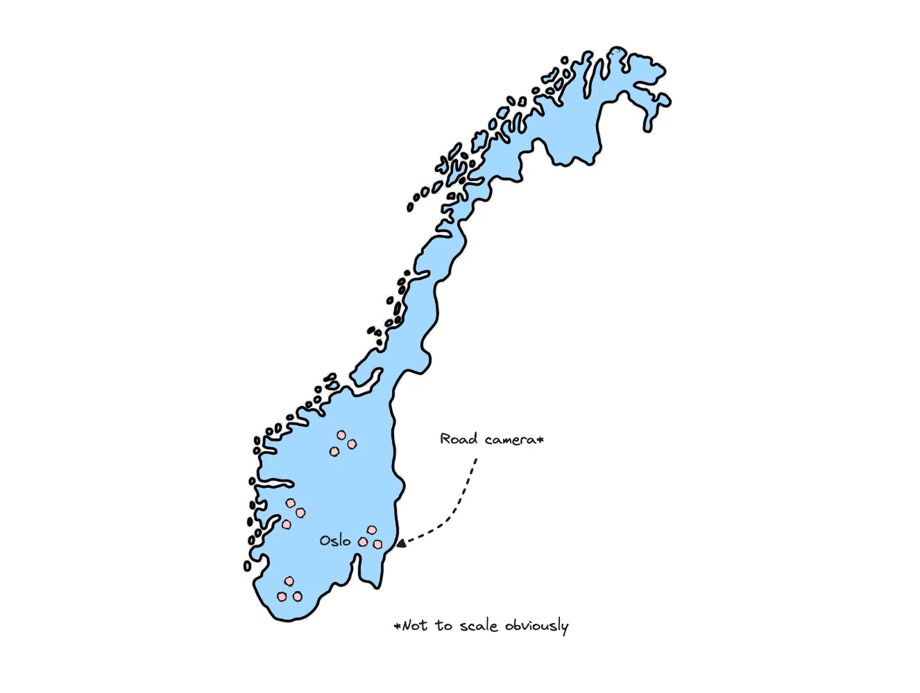
The task here is to classify traffic levels by public traffic cameras planted across the country in Norway. The cameras are almost updated in real-time, while the traffic API that is also available is updated hours after the traffic levels have been calculated.
The idea is to automate a process that checks the pictures of the cameras every minute, so we can estimate the traffic levels well before the API catches on.
The model I will build in this article was originally created for a media outlet in Norway but has been open-sourced, and you can find it here. It has been built using images from fifty out of the hundreds of public traffic cameras in Norway.
You’ll see me demonstrate how to use it below.
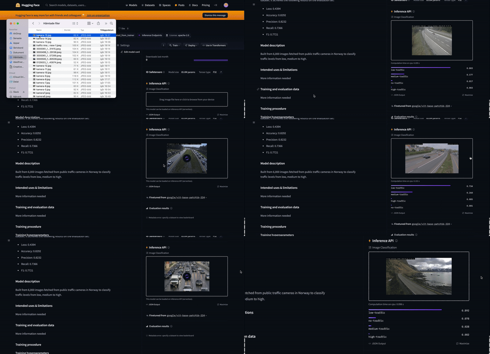
Do grab a picture from this or this camera and try it out to see how it does via the model page. As you can see, we can run it in CPU which will be quite cost-effective.
For due diligence though, I did check other options such as Google Traffic, which does provide us with good data for urban areas. However, we weren’t allowed to tap into it and it had very little data on areas outside of the city limits so it wasn’t a viable solution.
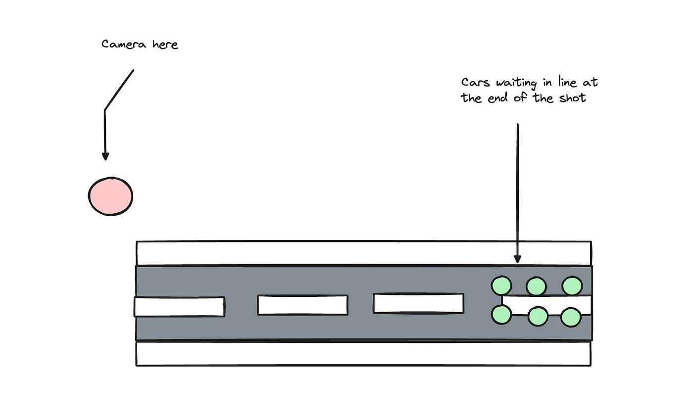
For Google Traffic, they estimate levels based on data that is shared by their user’s phones whereas we would do this manually, checking the public cameras for traffic levels with computer vision by estimating how many cars there are on the road or are waiting in line.
To understand the data we’re working with, do take a look at the dataset we’ll be using here.
As you can see, the images require us to interpret not just the amount of cars but whether they are waiting in line in various directions, in various different sceneries.
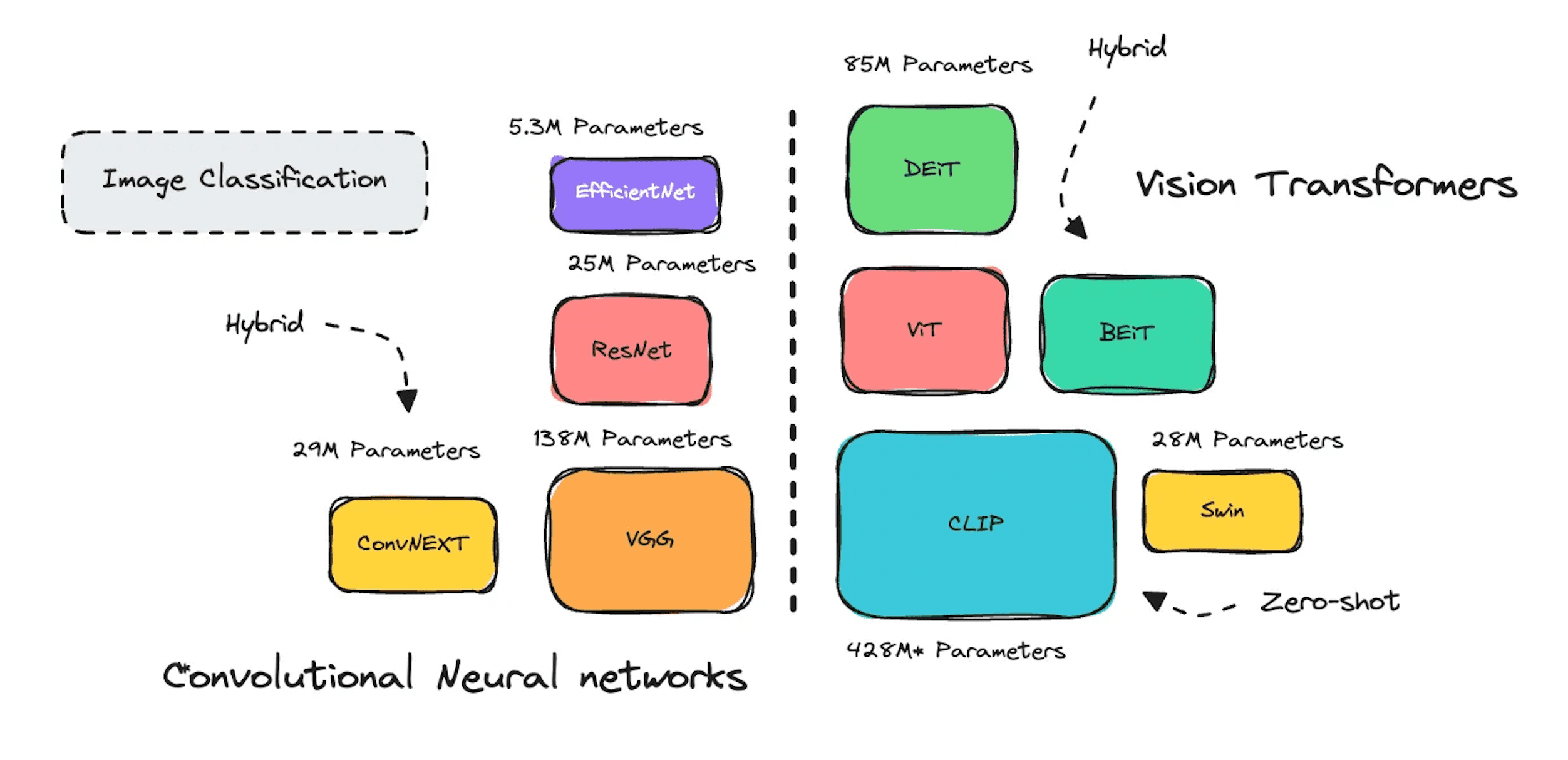
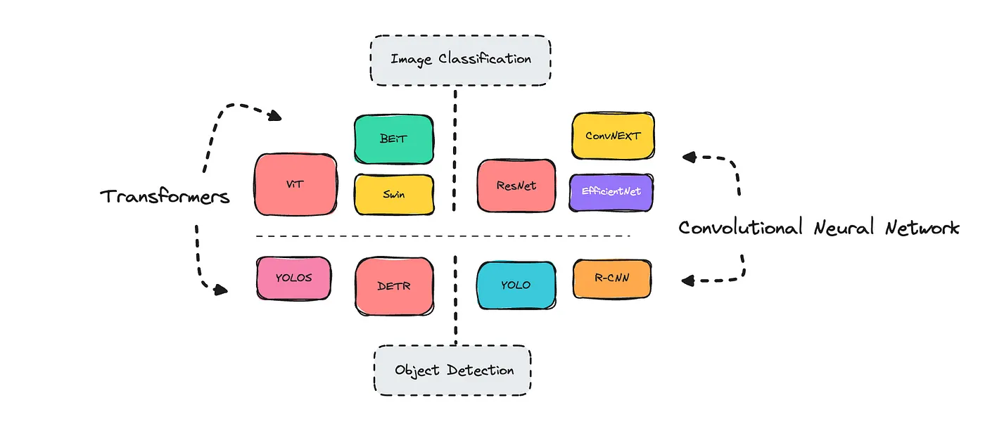
This article will go into the different architectures for the task — image classification — trying an older CNN model like ResNet and comparing it to newer models — ViT (Vision Transformer), Swin Transformer and ConvNEXT. I will also give a CLIP model a try in the introduction section.
I have not tried edge cases for this model, which you should do before you push it into production.
I’ve shared most cook books I’ve used in a Github repository that you can find here. These will help you prepare your image dataset to fine-tune for image classification, as well as how to train it with a ViT or a CNN model like ResNet.
I will go through the costs, the case and the results but feel free to scroll past the introduction if you want to go directly to the training section.
The Economics of Custom Models
If your mind is spinning right now with the question on why I would bother to build my own vision model versus just using a CLIP model or GPT-4 Vision, I’ll go through it briefly.
A CLIP model allows you to do zero-shot inference, which means you will provide it with the labels and it will do the best that it can with those labels to correctly estimate what is pictured in the image. For simpler cases, you should definitely go for a CLIP model. They are small enough that it won’t cost that much to host them.
Test out a ViT based CLIP model here by providing a few labels and an image it should classify.
However, with a CLIP model I wouldn’t be able to train the model to understand the nuances between medium and high traffic, and in most cases a high traffic image would get classified as medium traffic. It very much depends on how the model interprets the images.
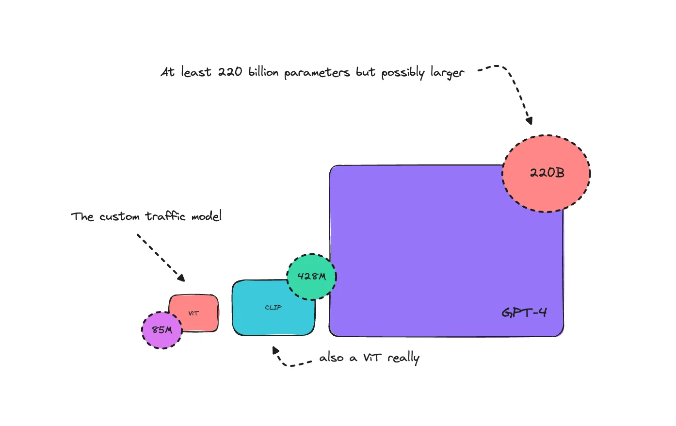
The CLIP model I linked to is also 5 times larger than the custom trained model that does better at the same task.
The same would happen if I used GPT-4 Vision; it wouldn’t always classify an image correctly that I would deem as high traffic. This is not accounting for cost, considering GPT-4 is vastly larger than a CLIP or a custom model.
If your first idea is to go for GPT-4 Vision, let’s first estimate the cost day to day if we were to monitor 50 to 150 cameras every minute, so you get an idea of the economics of using such a large model.
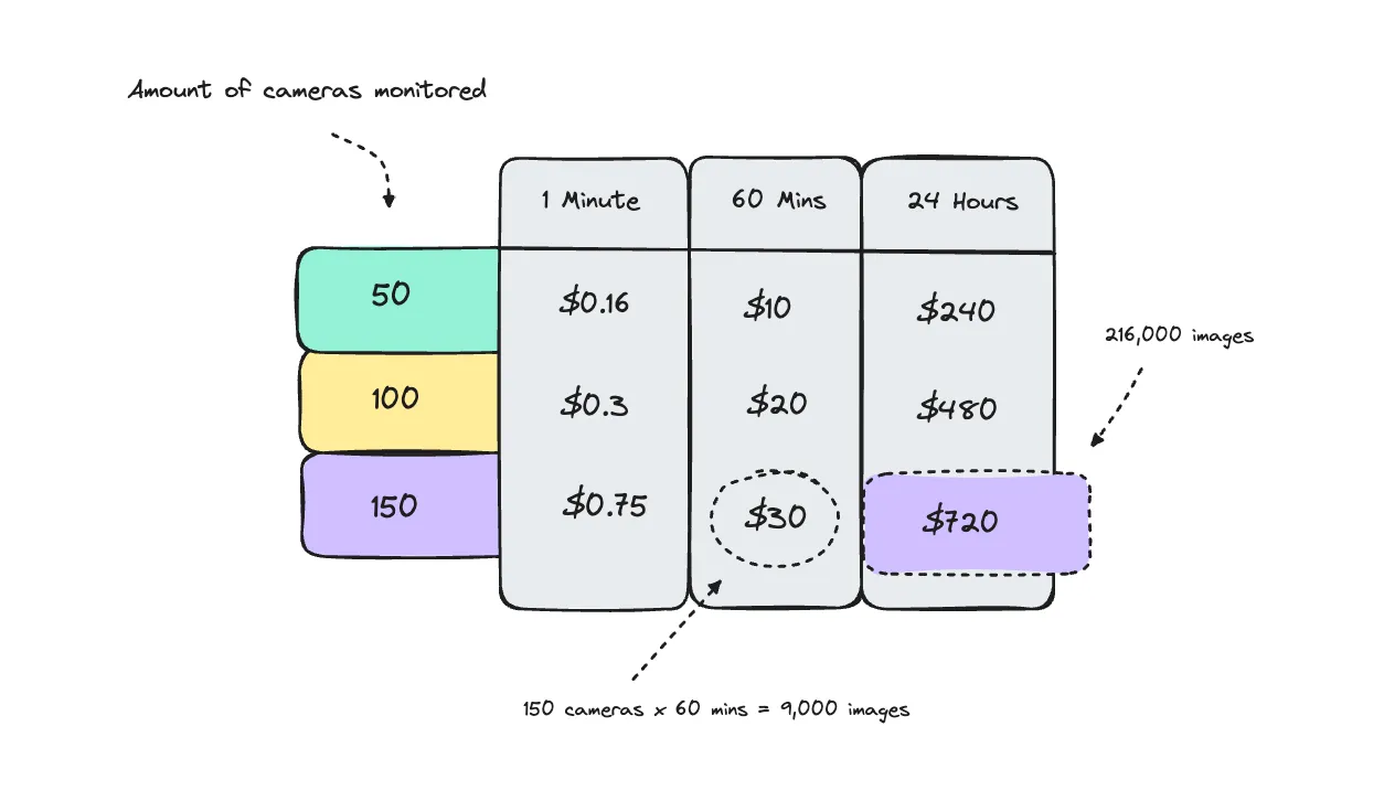
It seems dumb to visualize it, as most would never use these bigger models at such a high frequency but sometimes the economics of it isn’t taken into account. You need to consider the resources you are using and how to optimize those resources for the task at hand.
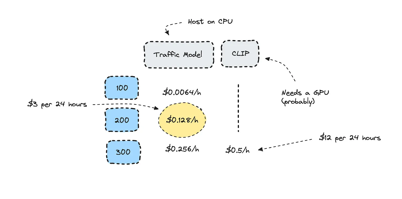
Let’s also look at the cost difference for hosting a CLIP at 428M parameters, or this custom built model at 85M parameters. The cost difference here is less, so in most cases it makes sense to use a CLIP.
Computer Vision
Computer vision is a subset of AI that trains computers to interpret and understand what we can “see.” Just as with natural language processing, we sort different areas into tasks, where we can choose different models and architectures to work with the task.
The most popular tasks within vision is image classification, object detection and segmentation.
The task I’m working with here is image classification, where I want a model to assign a label or a class to an image. If you’ve worked with text classification, it follows the same principles.
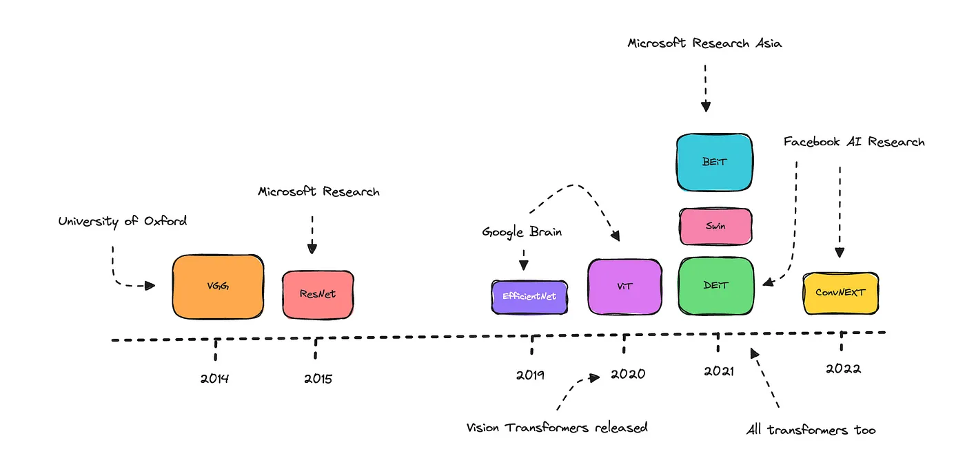
So for image classification, as with other tasks, you have several pre-trained models to choose from. So which one should you pick? Vision Transformers are fairly new and if you Google a bit you’ll find that most have been working with Convolutional Neural Networks (CNNs) such as ResNet.
The idea is that ViTs should be good at capturing global context and dependencies between distant parts of an image because of their self-attention mechanisms. However, the catch is that ViTs need a lot of data to perform. CNNs on the other hand, should be more efficient on smaller models and datasets. CNNs also have a proven track record.
A ViT will need a lot of data to perform, but it is a bit unclear if it is enough that the pre-trained model has been trained on enough data or if it needs a hefty amount for fine-tuning as well. If you listen to some people, it’s enough if it has been pre-trained on enough data.
The ideal thing is to test the different models, using a CNN — like ResNet — and a ViT model along with the newer models such as ConvNEXT and Swin Transformer on your dataset to see which does better.
I have done exactly this below, and you’ll see the metrics I achieved for each model.
If you are muddling through the same process, you’ll find cook books here to fine-tune for all different models.
The Use Case: Estimating Traffic Levels
Like I mentioned before, the use case we’re working with here is to classify the level of traffic from images from public road cameras in Norway.
These cameras are accessible to the public. You can freely download and use any photos and illustrations from the Norwegian Public Roads Administration.
I set up a script that would fetch images for certain times during the day and then I collected them into a folder that I later speed sorted whenever I had a few hours available.
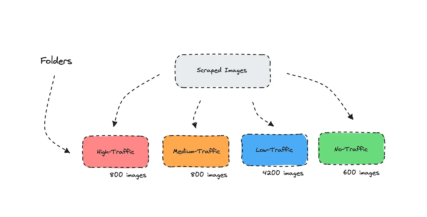
I did not have an unlimited amount of time, but in most cases you need more varied data to train with.
The finished dataset I used you’ll find here.
The problem with these images is that some roads consistently experience high traffic whereas other roads don’t. This then means that we’ll get a very skewed dataset as it’s rare that the roads will be packed with cars during all hours of the day. As you’ll notice, we have 4,200 images with low traffic and only 800 images with high traffic.
For this specific case, I did not need it to perform perfectly but I couldn’t have an image being classified as high traffic when it is clearly low traffic.
If it started generalizing it would be useless.
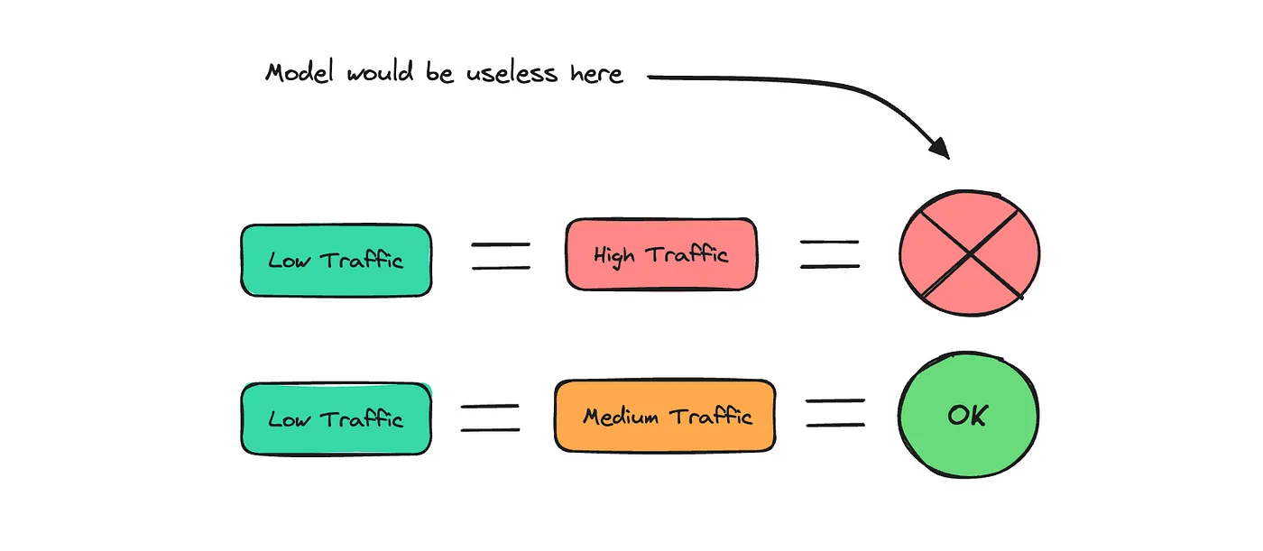
Nevertheless, if it sometimes classifies a high traffic image as medium traffic or a medium traffic image as a low traffic this would be less of a concern.
I’ll go through the results from the training directly, and if you’re keen you can check how I trained the model at the next section.
To train the model, I tested several models using 5e-5 as a learning rate with 5 epochs. I didn’t find that much of an improvement by increasing the number of epochs.
Surprisingly, a pre-trained standard ViT model did well on only 6,800 images.
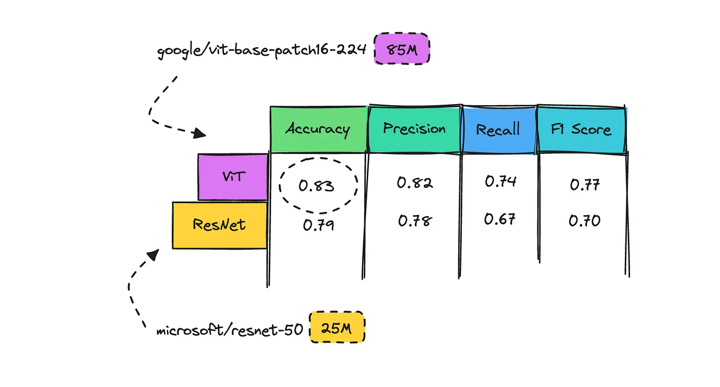
The ViT model is three times as large as the ResNet I used, but still quite small at 85M parameters.
The metrics show us that a ViT performed better on all metrics. Accuracy is the one we’re looking at the most, whereas the F1 will help us estimate how much our skewed dataset is a problem. A high F1 score means the model is not just guessing well for the common categories, but also doing a good job at correctly estimating the rare categories, such as medium and high traffic.
Furthermore, testing the model manually on new images, I found that the ResNet was more likely to classify a low traffic image as high traffic than a ViT, so this is why I primarily went with ViT along with the higher performance metrics.
The result could have primarily been because the ViT model was naturally larger but I needed a fairly large model for this case. I also wonder if a ViT is a better choice for these images where I need it to analyze the entirety of it to estimate traffic levels.
Continuing my experiment, I did not find that using a ConvNEXT or a Swin Transformer model gave me any positive change. They did surprisingly well though.
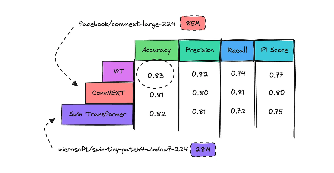
The metrics for ConvNEXT and Swin Transformer were good. However, testing the model on new images gave me inflated results where medium traffic images on high traffic roads were classified as high traffic, which was less of an issue with a standard ViT model.
This could have been a result of how my dataset had been filtered confusing the model with too many medium-traffic images in the high-traffic folder so I wouldn’t disregard these other models.
The metrics did not improve with a custom trainer to account for weight imbalances in the dataset when training a ViT. It performed about the same in practice with worse metrics. But there is probably room for improvement there as well.
Lastly, trying to balance the dataset manually by further introducing more high traffic images unfortunately gave me more generalized results on some high traffic roads — i.e. for high traffic roads it inflated the results regardless if the road was mostly empty — so for this case having an unbalanced dataset proved fruitful.
I did not try data augmentation to increase the size of the imbalanced dataset as I didn’t believe it would do any good.
Nevertheless, continuing to work on the dataset by setting up a script to pick up images over a longer period of time is a good idea. I would still keep it skewed to reflect the real thing though as I found it did better if it reflected reality.
Traffic images are notoriously difficult, as each camera will show a different scenario and a different scenery. Because of this I would also set up an algorithm later that would check how many images have been classified with high traffic between a few minutes to estimate how bad the traffic congestion is.
I would stress that this model is not battle-tested, and it would need to get further tested and trained.
Training the Model
I have provided several cook books so you can test both a CNN and ViT model using the HuggingFace trainer. You can tweak them as you go along, if needed.
The process to train this model, is the following.
- Prepare the dataset
- Preprocess the dataset
- Decide on your metrics
- Train the model
- Evaluate the model
Preparing a Dataset
When you work with image classification, you want to sort your images into folders. The folders will act as your labels, or categories.
From here it is easy enough to prepare and load your dataset so it can be pushed to the HuggingFace hub.
I usually mount my Google Drive in Colab and then simply load the dataset.
from google.colab import drive
drive.mount('/content/drive')
from datasets import load_dataset
dataset = load_dataset('imagefolder', data_dir=dataset_path)
You may want to check that the folders don’t have any corrupt files that will later be a problem when you train the model.
from PIL import Image
import os

dataset_path = '/content/drive/MyDrive/your-image-folder'

def verify_images(folder_path):
    for subdir, dirs, files in os.walk(folder_path):
        for file in files:
            filepath = os.path.join(subdir, file)
            try:
                with Image.open(filepath) as img:
                    img.verify()
            except (IOError, SyntaxError) as e:
                print(f'Corrupt image: {filepath} | Error: {e}')
                os.remove(filepath)

verify_images(dataset_path)
If you first do the check above, and delete any corrupt files, load the dataset after this.
Once you’ve loaded it, you can continue to split it into a training and validation set.
from datasets import load_dataset, DatasetDict

train_dataset = dataset["train"]

split_datasets = train_dataset.train_test_split(test_size=0.1, seed=42, stratify_by_column='label')

train_dataset = split_datasets['train']
val_dataset = split_datasets['test']

dataset_dict = DatasetDict({
    'train': train_dataset,
    'validation': val_dataset
})
We always use a training set to fit the model and a validation set to evaluate its performance.
When you’re done you can train it directly or you can push it to the HuggingFace hub to store for later training.
To push it to the hub you login like so.
!huggingface-cli login
repo_name = "username/traffic-camera-norway-images"
dataset_dict.push_to_hub(repo_name)
See the full script here to prepare your image data.
Find a Pre-Trained Model
Now as mentioned you’ll have to decide which pre-trained model you want to train. I will use a ViT here because it did best, but if you want to go for a ConvNEXT or a CNN model see other cook books here.
I’ll be going with the model vit-base-patch16–224 but you can try another one but just make sure you match the input specifications of each model, particularly the image size, when you preprocess your data later. I’ll explain it once we get to this part.
The vit-base-patch16–224 model has been pre-trained on the ImageNet-21k which should be enough data.
Open the Colab Notebook
If you’re good to go you can open this Colab notebook that I have already prepared.
At the start you’ll be able to set a few variables, your dataset url in HuggingFace, the pre-trained model you’ll fine-tune, the new model name as well as the learning rate, epochs and batch size.
dataset_url = "ilsilfverskiold/traffic-camera-norway-images"
model_checkpoint = "google/vit-base-patch16-224"
new_model_name = 'traffic-image-classification'
learning_rate = 5e-5
epochs = 5
batch_size= 32
The standard learning rate is 5e-5, and with 6800 images something like 5–10 epochs should be ideal. I didn’t find that it better after 5 epochs but it is up to you if you’d like to test it on more or less.
There should be a ton of information on this out there if you’d like to dig deeper.
I will skip a few sections, but do make sure you follow along in the Colab notebook.
##Preprocess Dataset
This pre-trained model we’re using has expectations on what the data should look like when we train it. Different models may have been trained with different image normalization standards.
So we load something called an image processor.
from transformers import AutoImageProcessor
image_processor  = AutoImageProcessor.from_pretrained(model_checkpoint)
We’ll use this one to normalize the images we’ll be training with so it will adjust the color channels to the same range and scale that the model was originally trained on.
We also resize the images to 256 pixels and then crop to the center to achieve a final size of 224x224 pixels, to follow the model’s input requirements.
Remember we picked a model with a resolution of 224x224 with vit-base-patch16–224.
from torchvision.transforms import (
    Compose,
    Resize,
    Normalize,
    CenterCrop,
    RandomHorizontalFlip,
    RandomResizedCrop,
    ToTensor,
)

normalize = Normalize(mean=image_processor.image_mean, std=image_processor.image_std)

train_transform = Compose([
    Resize(256),
    CenterCrop(224),
    RandomHorizontalFlip(),
    ToTensor(),
    normalize,
])

val_transform = Compose([
    Resize(256),
    CenterCrop(224),
    ToTensor(),
    normalize,
])

def apply_transform(examples, transform):
    examples['pixel_values'] = [transform(image.convert('RGB')) for image in examples['image']]
    return examples

def set_dataset_transform(dataset, transform):
    dataset.set_transform(lambda examples: apply_transform(examples, transform))

set_dataset_transform(dataset['train'], train_transform)
set_dataset_transform(dataset['validation'], val_transform)
The other random stuff we do, like random flips and other similar augmentation techniques are used to improve the robustness and generalization ability of machine learning models.
Lastly, the ToTensor() transformation converts PIL images to PyTorch tensors, formatting the data that is required by PyTorch models.
After this it is good to check that you have another field called pixel_values for each item with tensors.
dataset['train'][0]
Remember to follow along in the Colab notebook for the entire script.
Evaluation Metrics
You’ll also want to set up some evaluation metrics. You saw earlier that I was evaluating the model based on a few metrics although you always have to test it manually as well to see how it does with new data.
The most important metric you’re interested in is Accuracy, which measures the amount of predictions the model got right across all categories. This one you’ll see everywhere but there are other metrics you may want to use as well.
Precision measures how often predictions for a specific category are correct. So for my case, with traffic levels, high precision in a traffic category like ‘high traffic’ means that when the model predicts high traffic, it is usually right.
Recall tells us how well the model can identify all instances within a specific category, such as ‘low traffic’. High recall means the model is good at recognizing most low traffic situations.
The F1 Score is the weighted average of Precision and Recall.
When you have a skewed dataset like I have where some categories don’t show up as much as others, a high F1 Score is really good. It means the model is not just guessing well for the common categories, but also doing a great job at picking up the rare ones correctly.
To tweak the metrics I’ve set up for this use case, you can navigate to this part of the Colab notebook.
import numpy as np
from datasets import load_metric

accuracy_metric = load_metric("accuracy")
precision_metric = load_metric("precision")
recall_metric = load_metric("recall")
f1_metric = load_metric("f1")

def compute_metrics(eval_pred):
    logits, labels = eval_pred
    predictions = np.argmax(logits, axis=1)

    accuracy = accuracy_metric.compute(predictions=predictions, references=labels)
    precision = precision_metric.compute(predictions=predictions, references=labels, average='macro')
    recall = recall_metric.compute(predictions=predictions, references=labels, average='macro')
    f1 = f1_metric.compute(predictions=predictions, references=labels, average='macro')

    metrics = {
        "accuracy": accuracy['accuracy'],
        "precision": precision['precision'],
        "recall": recall['recall'],
        "f1": f1['f1']
    }
    return metrics
Model Training
From here we can prepare to train the model. Remember not to skip any parts in the notebook as I’m not going through all the steps here.
I’m using an L4 in Colab to train as I have a pro membership but this should work with a T4 as well, only the training may be slightly slower. Just remember to use a GPU.
Ideally you can keep the training arguments as is, and tweak epochs and learning_rate at the start.
args = TrainingArguments(
    f"{new_model_name}",
    remove_unused_columns=False,
    evaluation_strategy = "epoch",
    save_strategy = "epoch",
    learning_rate=learning_rate,
    per_device_train_batch_size=batch_size,
    gradient_accumulation_steps=4,
    per_device_eval_batch_size=batch_size,
    num_train_epochs=epochs,
    warmup_ratio=0.1,
    logging_steps=10,
    weight_decay=weight_decay,
    load_best_model_at_end=True,
    metric_for_best_model="accuracy",
    push_to_hub=False,
)
Do not remove remove_unused_columns as you’ll get an error. I have specified to not push it to the hub as I want to evaluate the model first.
We also set up the trainer with the prepared train and validation datasets.
trainer = Trainer(
    model,
    args,
    train_dataset=dataset['train'],
    eval_dataset=dataset['validation'],
    tokenizer=image_processor,
    compute_metrics=compute_metrics,
    data_collator=collate_fn,
)
If you’re satisfied you can go ahead and train the model.
train_results = trainer.train()

trainer.save_model()
trainer.log_metrics("train", train_results.metrics)
trainer.save_metrics("train", train_results.metrics)
trainer.save_state()
You’ll see the metrics for each epoch once it is training. What you’re looking for here is the training loss, which should consistently going down, while validation loss should do the same. I sometimes see it fluctuating, though it shouldn’t so do keep an eye on it.
Accuracy should obviously increase, as I mentioned when I talked about the evaluation metrics earlier.
Evaluate Model
Once it has finished training you can evaluate the final metrics.
metrics = trainer.evaluate()
trainer.log_metrics("eval", metrics)
trainer.save_metrics("eval", metrics)
My metrics weren’t stellar for this first run, but good enough for this case.
***** eval metrics *****
  epoch                   =     4.9215
  eval_accuracy           =     0.8292
  eval_f1                 =     0.7721 # good enough
  eval_loss               =     0.4394
  eval_precision          =     0.8232
  eval_recall             =     0.7366
The loss was quite high while the training loss a bit lower, which could indicate overfitting. I had better metrics for a few other models.
This is where you’ll want to also test the model on new data to see how it does. This model did better at new images than the other models that inflated the labels from medium to high traffic.
This could have been an issue with my validation set just not being large enough, and not representing real use cases.
So, I would also test it on various images to see how it does. For me this was easy enough as I ran it through a few new traffic images that I had stored in my Google Drive.
To do this save the model and then set up the pipeline with the new model.
trainer.save_model('new_model')
from transformers import pipeline
pipe = pipeline('image-classification', model='new_model')
Connect your Google Drive.
from google.colab import drive
drive.mount('/content/drive')
Then do some inference on the images you want.
from PIL import Image

image_path = '/content/drive/MyDrive/image_to_test.jpg' # path to your image

image = Image.open(image_path)

results = pipe(image)
results
Push to Hub (Optional)
If you’re decently satisfied, you can push the model to the Hub to use from there or to deploy it as an inference endpoint so you can use it in production.
You’ll see me doing this in the Colab notebook at the end. The notebook should help you from start to finish.
Testing the Model
Now we can test the model in the hub using the Inference API and see how it does.
I’m always terrified that I’ll find something I don’t want to see so I haven’t yet tried any edge cases yet, like a picture with a bunch of trees in the middle of the screen.
Nevertheless, we know it might miss a few high traffic images but at least it’s not classifying low traffic as high traffic.
I open sourced the model I created here which is probably far from perfect but you are very welcome to use it.
I also open sourced the first dataset that you can find here.
Hopefully this proved resourceful and you get some inspiration for your next project.
❤